1. Introduction

In this post, I want to talk about stochastic gradient estimators and, along the way, introduce my master thesis. You probably have heard about RLHF, which is an application of Reinforcement Learning to align pretrained Large Language Models with human preferences (to a reward model modelling human preferences to be more specific).

Usually in RLHF, after obtaining the reward model you would train your LLM using PPO. Another valid approach, which was shown to improve on PPO¹, is to use a very old algorithm from RL called the REINFORCE algorithm².

\[\mathbb{E}_{x \sim D, y \sim \pi_\theta(\cdot|x)} \left[ R(y, x) \nabla_\theta \log \pi_\theta(y|x) \right]\]

Here \( x \) is the prompt, \( y \) is the continuation generated by the LLM \( \pi_\theta(y|x) \), whose parameters \( \theta \) we are trying to optimize. The equation above describes the gradient we use to maximize the reward in the form of an expectation. By doing a Monte-Carlo approximation, that is by sampling, we can obtain a stochastic gradient estimate. In theory, we only need one sample to obtain a gradient (This is also what they use in ¹).

Actually the above formulation of the form of sampling from a distribution \( p_\theta(x) \) and evaluating its score \( R(x) \) is a very general formulation encountered widely, f.e. in episodic reinforcement learning, where \( x \) is a trajectory and \( R(x) \) is the sum of rewards along the trajectory.

\[\mathbb{E}_{x \sim \pi_\theta(\cdot)} \left[ r(x) \right]\]

Other instances include black-box optimization, where \( x \) is a point in the search space and \( r(x) \) is the value of the objective function at that point, or evolutionary algorithms, where \( x \) is a candidate solution and \( r(x) \) is the fitness of that solution³. In all these cases we are estimating the gradient through sampling. The question is, how can we do this more efficiently? That is, with as few samples as possible while maintaining a good quality of the gradient. With quality I mean that the gradient should point in the direction of the true gradient (unbiased), and that the variance of the gradient should be low. This is important because the quality of the gradient directly influences the convergence speed of the optimization algorithm (but also if it converges at all). To find a good gradient estimator, that was the goal of my master thesis.

2.REINFORCE and Measure Valued Derivative Gradient Estimators

The REINFORCE gradient estimator, which we saw above, is easy to undestand, implement and unbiased, that is given enough samples it will converge to the true gradient. However, it has a high variance, which makes it slow to converge. This is because the gradient is multiplied by the reward, which can be very large or very small, leading to a high variance.

We can derive the REINFORCE estimator as follows

\[\nabla_{\theta} \mathbb{E}_{x \sim p_\theta(\cdot)} \left[ R(x) \right] = \int \nabla_{\theta} p_\theta(x) R(x) dx = \int \nabla_{\theta} p_\theta(x) \cdot \dfrac{p_\theta(x)}{p_\theta(x)} R(x) dx = \int \nabla_{\theta} \log p_\theta(x) p_\theta(x) R(x) dx = \mathbb{E}_{x \sim p_\theta(\cdot)} \left[ \nabla_{\theta} \log p_\theta(x) R(x) \right]\]

where we used the identify \( \dfrac{\nabla_{\theta} p_\theta(x)}{p_\theta(x)} = \nabla_{\theta} \log p_\theta(x) \) and the interchangeability between integration and derrivative. This quantity \( \nabla_{\theta} \log p_\theta(x) \) is also known as the Score Function (SF) in information theory. We use the SF and REINFORCE interchangeably.

On the other hand, we have the Measure-Valued Derivative (MVD) Estimator. The MVD is based on a mathematical theorem that formulates the derivative of a distribution wrt its parameters as a difference between two distribtions. This formulation has been first introduced by Pflug in 1989 ⁴, which went by relatively unnoticed in the machine learning community until it was picked up by Rosca et al in 2020 ⁵ and my supervisor Joao ⁶. Both have realized the potential of this underexplored gradient estimator and have shown that it leads to a lower variance than the Score Function Estimator (SF) for the cases of Bayesian Inference and Policy Gradients.

The MVD estimator is based on the following decomposition given by Pflug⁴

\[\nabla_{\theta} p_\theta(x) = c_\theta ( p_{\theta}^{+}(x) - p_{\theta}^{-}(x) )\]

where each distribution has its own characteristic decomposition triplet \( (c_\theta, p_{\theta}^{+}, p_{\theta}^{-}) \). For a Gaussian distribution for example, the decomposition is given by

\[( \frac{1}{\sigma \sqrt{2\pi}}, \theta + \sigma \mathcal{W}(2, 0.5), \theta - \sigma \mathcal{W}(2, 0.5) )\]

where \( \mathcal{W}(2, 0.5) \) is a Weibull distribution with shape parameter 2 and scale parameter 0.5. More decompositions can be found in my thesis or any other paper on MVDs. The MVD estimator is then given by

\[\nabla_{\theta} \mathbb{E}_{x \sim p_\theta(\cdot)} \left[ R(x) \right] = c_{\theta} \left( \mathbb{E}_{x \sim p_\theta^{+}(\cdot)} \left[ R(x) \right] - \mathbb{E}_{x \sim p_\theta^{-}(\cdot)} \left[ R(x) \right] \right)\]

Thus the MVD estimator is based on the difference between two expectations. It is unbiased and has a lower variance than the SF estimator. However, the big caveat here is that this decomposition and sampling has to be done for every dimension of the parameter space. The sample complexity is thus \( \mathcal{O}(2D) \) where \( D\) describes the parameter dimensionality. For comparison the SF estimator has \( \mathcal{O}(1) \). This is a big drawback, but is it worth it? Let’s find out!

3. Comparing SF and MVD

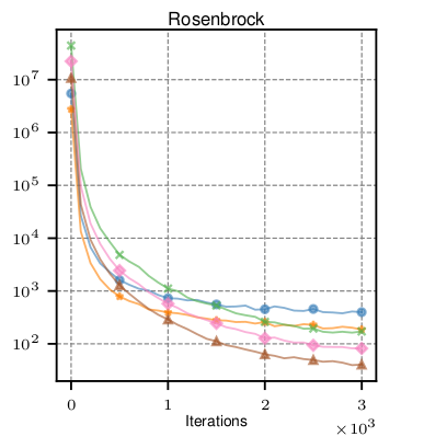
We can now compare both estimators in a simplified environment to check their gradient quality. Here we can use cost functions from the black-box optimization community such as the Rosenbrock function. The Rosenbrock function is a non-convex function that is used as a performance test problem for optimization algorithms. It is defined as

\[f(x, y) = (a - x)^2 + b(y - x^2)^2\]

What we are looking for is a gradient that points in the direction of the true gradient and has a low variance using as few samples as possible.

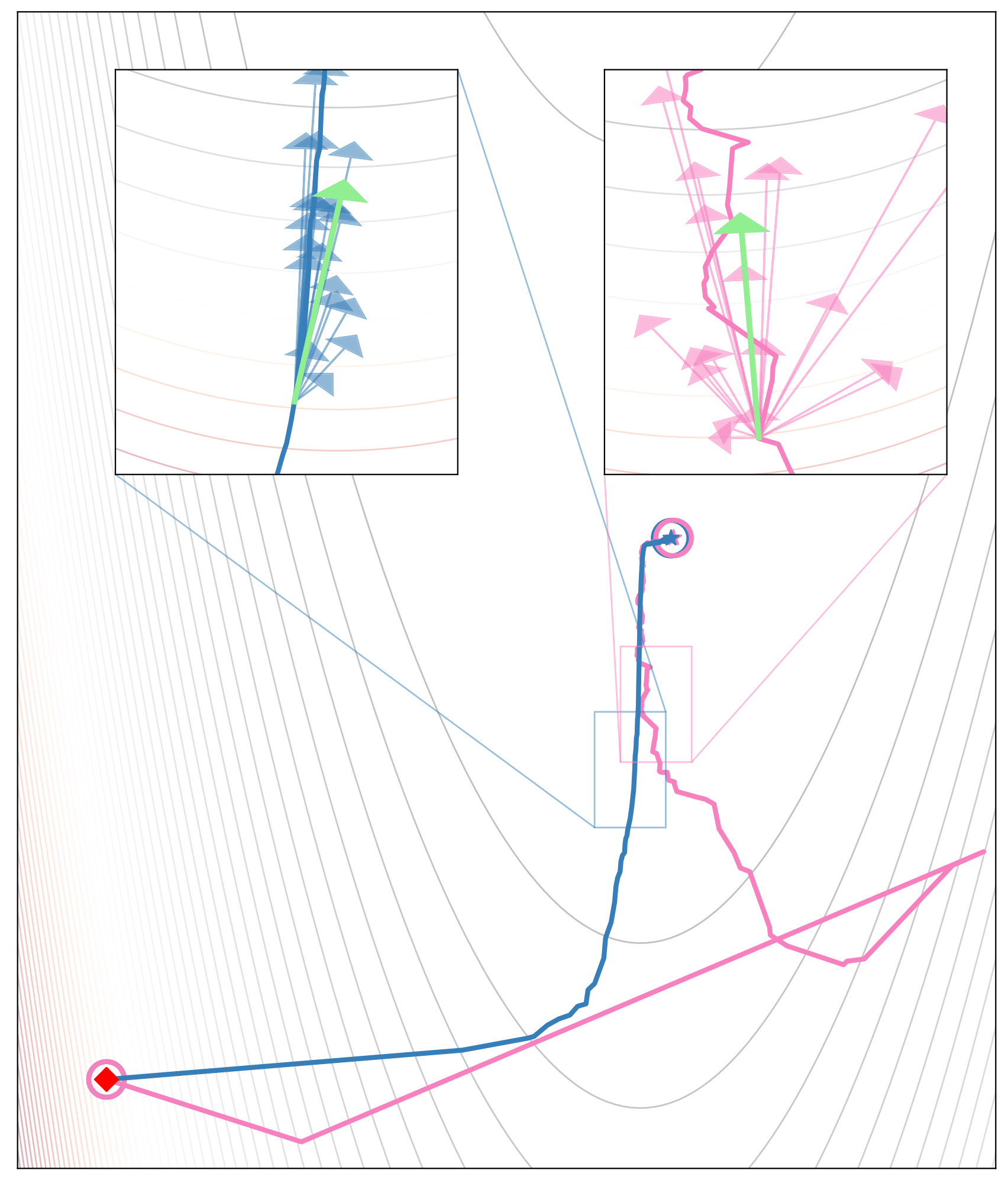
Below we can see each gradient sample ploted as vector in a 2D parameter space. The true gradient is given by the green vector. The SF gradient is given by the pink vectors and the MVD gradient is given by the blue vectors. We can see that the MVD gradient points more in the direction of the true gradient and has a lesser variance in direction and magnitude than the SF gradient.

Eventhough the MVD estimator seems to have a lower variance than the SF estimator, it is not a silver bullet. The MVD estimator has a higher computational cost than the SF estimator with its \( \mathcal{O}(2D) \) complexity. With growing number of dimensions, the MVD estimator will become more and more expensive to compute, and the SF estimator with its \( \mathcal{O}(1) \) will become more and more attractive, as using more samples will naturally reduce the variance of the estimator.

Below you can see the variance of the SF and MVD estimator with varying number of samples \( N \) in \( 10 \) dimensional space. We can see that using the same budget of samples, the advantage of the MVD estimator diminishes with growing number of dimensions.

6. Combining SF and MVD

Can we combine the advantages of both estimators? Yes, we can! We can use the MVD estimator to estimate the gradient in the most important dimensions and the SF estimator to estimate the gradient in the less important dimensions.

In general to build such a hybrid estimator, we need the following ingredients:

• A measure of importance for each dimension
• A strategy to combine the estimators

All this with the goal of reducing the variance of the combined estimator. For the measure of importance we can use the empirical variance of the SF estimator and select the dimensions with the highest variance to be combined with the MVD estimator. For the strategy to combine the estimators, we can use a convex combination of the MVD and SF estimators, where the weights are given through their respective variance. The hybrid estimator called Convex Combined MVD (CCMVD) is then given by:

\[\hat{g} = \dfrac{\sigma_{\text{SF}}^2}{\sigma_{\text{SF}}^2 + \sigma_{\text{MVD}}^2} \hat{g}_{\text{SF}} + \dfrac{\sigma_{\text{MVD}}^2}{\sigma_{\text{SF}}^2 + \sigma_{\text{MVD}}^2} \hat{g}_{\text{MVD}}\]

7. Results

We can now validate our ideas on real reinforcement learning problems. For this we utilize the MuJoCo environment⁷. We can first see if the CCMVD estimator can really reduce the variance relative to REINFOCE estimator using the same budget, and if using another SF estimator for convex combination might lead to a simlar level of variance reduction (which we call CCSF here). The sampling budget of the convex combined estimators is given through

\[2 (N + M \cdot K)\]

where \( N, M , K \) are the number of SF samples, number of MVD samples and the number of selected MVD dimensions respectively.

Below we can see the variance reduced at the selected dimensions for variour choices of \( (N , K , M) \). The variance reduction measured as the relative difference to a SF estimator using the same sample budget \( 2 (N + M \cdot K) \). The parameter dimensions of the environments are:

• swimmer : 16
• hopper : 33
• half_cheeta : 102
• walker : 102

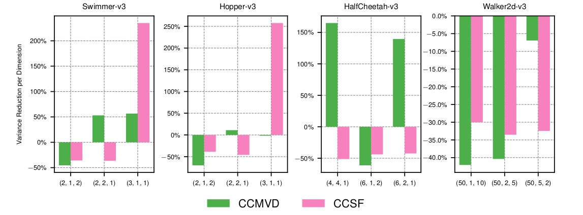
We see that variance at the chosen dimensions is reduced for all cases when the number of samples for the MVD M is larger one. In such cases, variance reduction with the CCMVD is mostly more effective than CCSF. However, as the number of selected dimensions K increases, the number of function evaluations increases with \( 2KM \) . By taking more samples for the CCSF to adjust for the increase of function evaluations, an increased variance reduction for the CCSF is observed.

As such the CCMVD estimator is more effective in reducing the variance of the gradient, but the positive effect dimiminishes with growing number of selected dimensions.

Next let us take a look at the reward curves. These were obtained using an average of 5 runs. \( V1, V2\) denote different ways of estimating the covariance matrix in the CCMVD estimator, and Random means that the dimensions are selected randomly. These are compared to a SF estimator using the same sample budget.

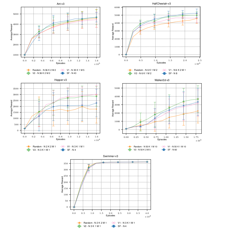
We can see that the reduction in variance does not necessarily lead to a better performance. The CCMVD estimator is in three out of five environments outperformed by the SF estimator. For the hopper enviromnet, where it performs best, the CCMVD estimator does not actually show a significant reduction in variance, as indicated by the above plots.

8. Conclusion

In this post, we have seen that the MVD estimator has a lower variance than the SF estimator, but it has a higher computational cost. We have also seen that the CCMVD estimator can reduce the variance of the gradient, but this does not necessarily lead to a better performance. The CCMVD estimator is more effective in reducing the variance of the gradient, but the positive effect diminishes with growing number of selected dimensions. Potential future work can be done in exploring better ways to select the dimensions and to combine the estimators.

---